Niels Bohr
In 1913 Niels Bohr introduced his model of the Hydrogen atom. No doubt influenced by Rutherford’s work, he suggested that the atom consists of a central, resting proton (nucleus) with an electron orbiting in a circle of radius re. According to the latest information on the Internet, in the atom’s lowest energy state, re1 (the ground state radius of the electron’s orbit), is re1= 5.291772 × 10⁻¹¹ meters. And the value for the electron’s inertial mass is |me|= 9.10938356 × 10⁻³¹ kg.
According to Coulomb, F1, the force exerted on the ground state electron by the proton, has the magnitude F1=q2/4πεo(re12). And according to Newton F1=(me)(ve12)/(re1), where ve1 is the electron’s speed. Equating these two expressions for F1, we find that ve1=q/(4πεo(re)(me))1/2 =2187691 meters/sec. It might be said that in a circle of radius~.5e-10 meters this is a “blinding” speed!
Bohr postulated that the electron’s angular momentum, L=(me)(ve)(re), equals =Nh/2π, where h=6.626068e-34 is Planck’s constant. (N=1, 2, 3…, with N=1 being the lowest ground state.) Thus according to Bohr’s postulate the most probable value for the ground state ve1 is 2187691 meters/sec, in agreement with the above.
Let us now critically consider Bohr’s assumption that the proton is at rest at the origin of an inertial rectangular coordinate system. Looking down from the positive z-axis, we imagine that the electron is initially at (-re,0,0) and is circling CCW around the origin. This would mean that at any given instant the entire atom’s momentum would simply equal the electron’s momentum. But the electron’s momentum varies in direction from moment to moment. Yet in Bohr’s model the atom’s total momentum is zero at any given moment. The only way this condition can be satisfied is if the proton is not actually at rest. Assuming the atom’s center is at rest at the origin, the proton must rotate CCW around the atom’s center quite as the electron does. And the electron and proton must be diametrically opposed at every instant. Of course the proton’s orbital radius would be less than that of the electron, owing to the proton’s mass being greater than the electron’s. Together the two should orbit CCW around the origin at a common angular frequency of ω=ve/re.
But our critique of Bohr’s model is not yet done for the following reason: the electron should radiate energy, since any charged particle going around a circular path radiates. Indeed Lorentz had found that a charge, going in a circle of radius r and at speed v, should experience a “radiation reaction” force opposite at any moment to the direction of v. In the Bohr atom the formula for this force is FRadReact=q2ω3(re)/(6πεoc3). If this force is not counteracted, then the electron should radiate and spiral into the proton. However, if it is counteracted by a component of the electric force from the proton , then it should not radiate. It should continue to travel at a constant speed in a circle.
What might be the explanation for the needed counteraction to FRadReact acting on the orbiting electron? A magnetic force engendered by a nonzero Bz would act perpendicular to v. It must be a component of an acting electric force engendered by the rotating proton.
Now unknown to Bohr, later theorists worked out the formula for the electric field of a charge whose kinetic history is known. This formula entails terms such as the source charge’s retarded velocity and acceleration, which pertain to a time prior to the electric force on some distant charge. The key to this phenomenon is that electromagnetic fields are not instantly felt at distant points. Their influence travels at the speed of light from source charge to subject charge. The field, felt by a subject charge at time t, is a function of kinematical variables at the source charge at some earlier time. As mentioned earlier, the formula for the radiation reaction force, acting on the Bohr model electron at time t=0, is FRadReact=q2ω3(re)/6πεoc3. And the formula for the proton-engendered electric force acting on the electron is the negative of FRadReact! This force provides the needed counteraction to FRadReact. If the sum of these two forces is zero, then the net radiation emitted by the electron is zero.
We may determine where the proton must have been at the retarded time by “inching up” to values for L and θ using a computer (L is not angular momentum. See Fig. 1 for a schematic.) Fig. 1 is followed by a Python program that does the inching up. Note that the radius of the proton’s orbit has been greatly exaggerated in the schematic for clarity.
It is worth mentioning that Bohr’s postulate, LN=Nh/2π, does not apply to H atom protons. The formula that works in the proton case is Lp=N(hp)/2π, where the constant ‘hp’ is a companion to h. hp has the value hp = 2πLp/N = 3.608669e-37 = h(me/mp).
Figure 1
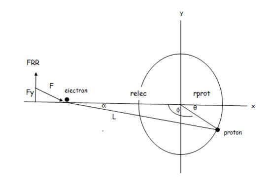
The Bohr Atom at a Typical Retarded Time
Inching up program:
import math
c=2.99792458e8  #Speed of light
h=6.626068e-34    #Planck constant
eps0=8.85418782e-12    #Permittivity constant
q=1.60217662e-19    #Elementary charge
ElectronMass=9.10938356e-31   #Electron rest mass
me=ElectronMass
ProtonMass=1.6726219e-27    #Proton rest mass
mp=ProtonMass
ElectronOrbitRadius1=.529177211067e-10
re1=ElectronOrbitRadius1
ve1=q/math.sqrt(4*math.pi*eps0*me*re1)
L1=me*ve1*re1
print('L1=',L1)
L1=h/(2*math.pi)
print('L1=',L1)
input("OK?")
#Any of the lowest 10 energies can be computed.
N=0
while N<=10:
    N=int(input('level=?(>10 to exit) '))
    if(N<11):
        print('Computing level ',N)
        #ElectronOrbitRadius=N**2*ElectronOrbitRadius1    #N'th level electron orbit radius
        L=N*L1
        ve=q**2/(4*math.pi*eps0*N*L1)
        print('ve1=',ve1,', ve=',ve)
        input('OK?')
        #ElectronSpeed1=h/(2*math.pi*ElectronMass*ElectronOrbitRadius1)            #Bohr rule
        ve=h/(2*math.pi*me*re1*N)
        print('ve=',ve)
        input('OK?')
        #ElectronKineticEnergy1=ElectronMass*ElectronSpeed1**2/2           #Electron kinetic energy
        #ElectronKineticEnergy=ElectronMass*ElectronSpeed**2/2
        re=N*L1/(me*ve)
        taue=2*math.pi*re/ve
        nue=1/taue    #Orbital fequency
        omega=2*math.pi*nue    #Angular frequency
        vp1=me*ve1/mp #total momentum=0
        vp=me*ve/mp
        rp1=vp1/omega
        rp=vp/omega
        #ProtonKineticEnergy=ProtonMass*ProtonOrbitalSpeed**2/2
        #PE=-q**2/(4*math.pi*eps0*(ElectronOrbitRadius+ProtonOrbitalRadius)) #Potential energy
        #TotalEnergy=ElectronKineticEnergy+ProtonKineticEnergy+PE    #Total energy of atom
        maxN=1e8    #Maximun number of iterations in orbital computation
        #DelayedTime=(ElectronOrbitRadius1+ProtonOrbitalRadius1)/c
        DelayedTime=(re+rp)/c
        dt=-DelayedTime/maxN    #Time increment
        loopN=-1
        theta=0.    #See diagram
        RadReactF=q**2*omega**3*re/(6*math.pi*eps0*c**3)
        RetardedProtonSpeed=vp    #Proton travels at constant speed
        ar=RetardedProtonSpeed**2/rp
        Fy=0.    #Initial trial force of proton on electron
        #Find parameters when forces on electron sum to zero
        while RadReactF+Fy>=0:
            loopN=loopN+1
            #If infinite loop, Print params and exit by clicking X in display
            if loopN>maxN:
                print('Possible infiite loop.')
                print('loopN, RadReactF, Fy',loopN,'; ',RadReacF,', ',Fy)
                print('Abort by clicking X in your display.')
                input('OK?')
            #If necessary, keep 'inching up’ to loop termination condition.
            RetardedTime=-loopN*dt
            theta=omega*RetardedTime
            RetardedVelocityX=vp*math.sin(theta)    #See diagram
            RetardedVelocityY=vp*math.cos(theta)
            RetardedAccelerationX=-(vp**2)/rp*math.cos(theta)
            RetardedAccelerationY=vp**2/rp*math.sin(theta)
            L=math.sqrt((re+rp)**2-(rp*math.sin(theta))**2)    #See diagram
            alpha=math.atan(rp*math.sin(theta)/L)
            Lx=-L*math.cos(alpha)
            Ly=L*math.sin(alpha)
            #Compute electric field at electron (see Griffith's text)
            ux=c*Lx/L-RetardedVelocityX
            uy=(c*Ly/L-RetardedVelocityY)
            u=math.sqrt(ux**2+uy**2)
            ux=-u*math.cos(alpha)
            uy=u*math.sin(alpha)
            Ey=q/(4*math.pi*eps0)*L/(Lx*ux+Ly*uy)**3
            Ey=Ey*(uy*(c**2-RetardedProtonSpeed**2)-(Lx*(ux*RetardedAccelerationY-uy*RetardedAccelerationX)))
            Fy=-q*Ey    #Interactive force on electron
        #When Fy+RadiationReactionForce=0, display results.
        L=math.sqrt((re+rp)**2-(rp*math.sin(theta))**2)    #See diagram
        alpha=math.atan(rp*math.sin(theta)/L)
        Lx=-L*math.cos(alpha)
        Ly=L*math.sin(alpha)
        print("L=",L)
        print("alpha=",alpha)
        print("Lx=",Lx)
        print("ve=",ve," vp=",vp," rp=",rp)
        print(N*h/(2*math.pi*me*re*ve)) #should be 1.
        print('RadReactF,Fy= ',RadReactF,', ',Fy)
        #Do another level.
#Reference: Griffiths, Introduction to Electrodynamics.